Monopoles and confinement
Direct link to article: arxiv.org
A magnetic monopole is a hypothetical elementary particle that is an isolated magnet with only one magnetic pole. The situation is very much like in the Ginzburg-Landau theory for the superconductor. In this theory an electromagnetic field interacts with a fundamental scalar field describing Cooper pairs. The latter are bound states of two electrons with opposite momentum and spin. As bosonic objects they can fall into the same quantum state resulting in one scalar field φ. The potential of the scalar field is of the Mexican-hat form with temperature-dependent coefficients. In the low temperature phase the symmetry is broken and the photons become massive. That means if a magnetic field enters the superconductor at all, it does so in flux tubes. Performing an Aharonov- Bohm experiment around such a tube leads to a flux quantum (this is a quote from an excellent article by Gerard ’t Hooft on Monopoles, Instantons and Confinement).
We consider a STIRAP system with the Schrödinger equation \begin{equation} i\hbar\frac{\partial}{\partial t} \Psi(R,t) = H\Psi(R,t), \end{equation} where the Hamiltonian is
\begin{equation} H = \left[ \matrix{ T+V_1(x) & \lambda_1(t) & 0 \cr \lambda_1(t) & T+V_2(x) & \lambda_2(t) \cr 0 & \lambda_2(t) & T+V_3(x) \cr } \right]. \end{equation} \(T\) is a kinetic energy, \(V_i \sim x_i^2 \) is a potential energy of an harmonic oscillator and \(\lambda_i\) is a coupling between the states. The couplings \(\lambda_1(t) \) and \(\lambda_2(t) \) are applied in the counterintuitive order.
A visual illustration of the population transfer from the level 1 to the level 3 is shown in the following figures:
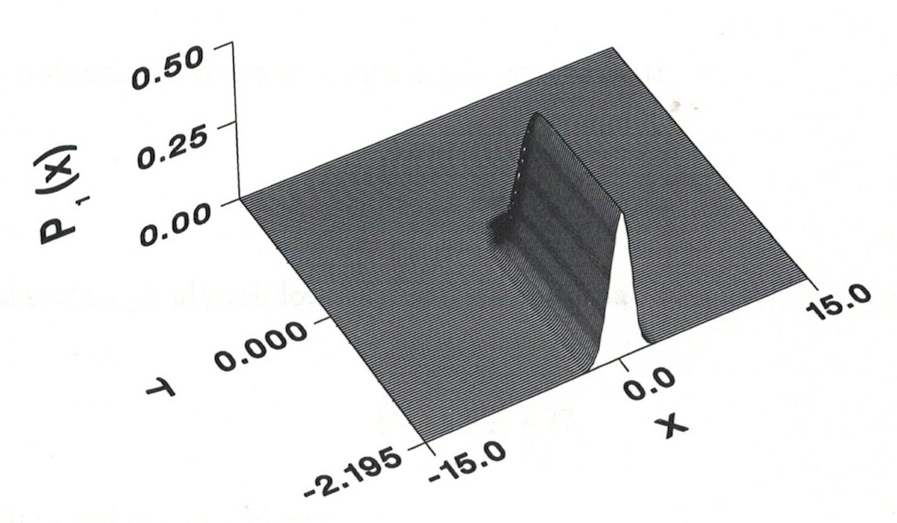
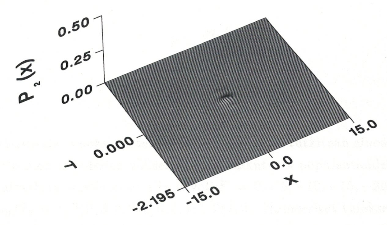
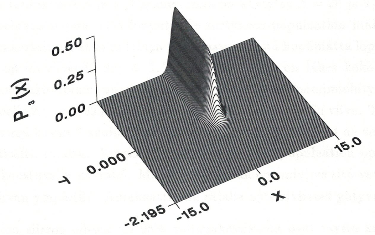
Level 2 is needed in the transfer and a small amount of population is visiting on the state, see Figure 2.
As it is discussed in the reference paper, when the pulse areas are finite, there exists a pair of monopoles with opposite charges in the system. A visual illustration of this situation is shown in the enclosed figure.
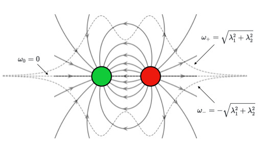
The figure shows the time evolution of the eigenvalues \(w_0 \) and \(w_{\pm} \) in the eigenspace. The monopoles are drawn in red and green in the figure. They locate at the origin of the parameter space.
More details and discussions can be found from the reference paper.
More topics on Quantum computing.